Improbably High Returns
Most people – even those with some knowledge of mathematics – would probably intuitively assume that the expected value of a random variable, such as the rate of return on an equity portfolio, is a particularly probable value. However, this is not the case. Yet this common misconception can have serious consequences – especially where risky investments are concerned.
Expected gains in the St Petersburg lottery
The so-called St Petersburg lottery is a paradox that has intrigued academics – including those at the original Russian Academy of Sciences in St Petersburg – ever since the early 18th century. This lottery involves tossing a coin – which features ‘heads’ on one side and ‘tails’ on the other – until tails appears for the first time; the lottery is then over. If tails appears on the first toss, the player wins two roubles; if it appears on the second toss, he wins four roubles; if it appears on the third toss, he wins eight roubles, and so on. What would be an appropriate price to pay to enter this lottery?
The first obvious answer that possibly springs to mind is the mathematical expected value, in other words the probability-weighted mean. The probability of tails appearing on the first toss is ½, on the second toss it is ¼ and, as a general rule, on the k-th toss it is (½)k. The probability-weighted value (expected value) of each individual possible payout amount 2k is therefore always 1 = 2k∙ (½)k. If we then aggregate this across n tosses of the coin, we get n as the expected total payout for up to n tosses. Because the coin can, in principle, be tossed an unlimited number of times, the expected gain is infinitely large. This example is often used in mathematics to demonstrate that there are probability distributions with infinitely large expected values.
However, hardly anyone would be prepared to pay anything like an infinitely high price to enter this lottery. One might reasonably object that in reality it is not even possible to toss a coin an infinite number of times. But this does not turn out to be the main problem when considering expected values.
The risk of not achieving the expected gain is very high
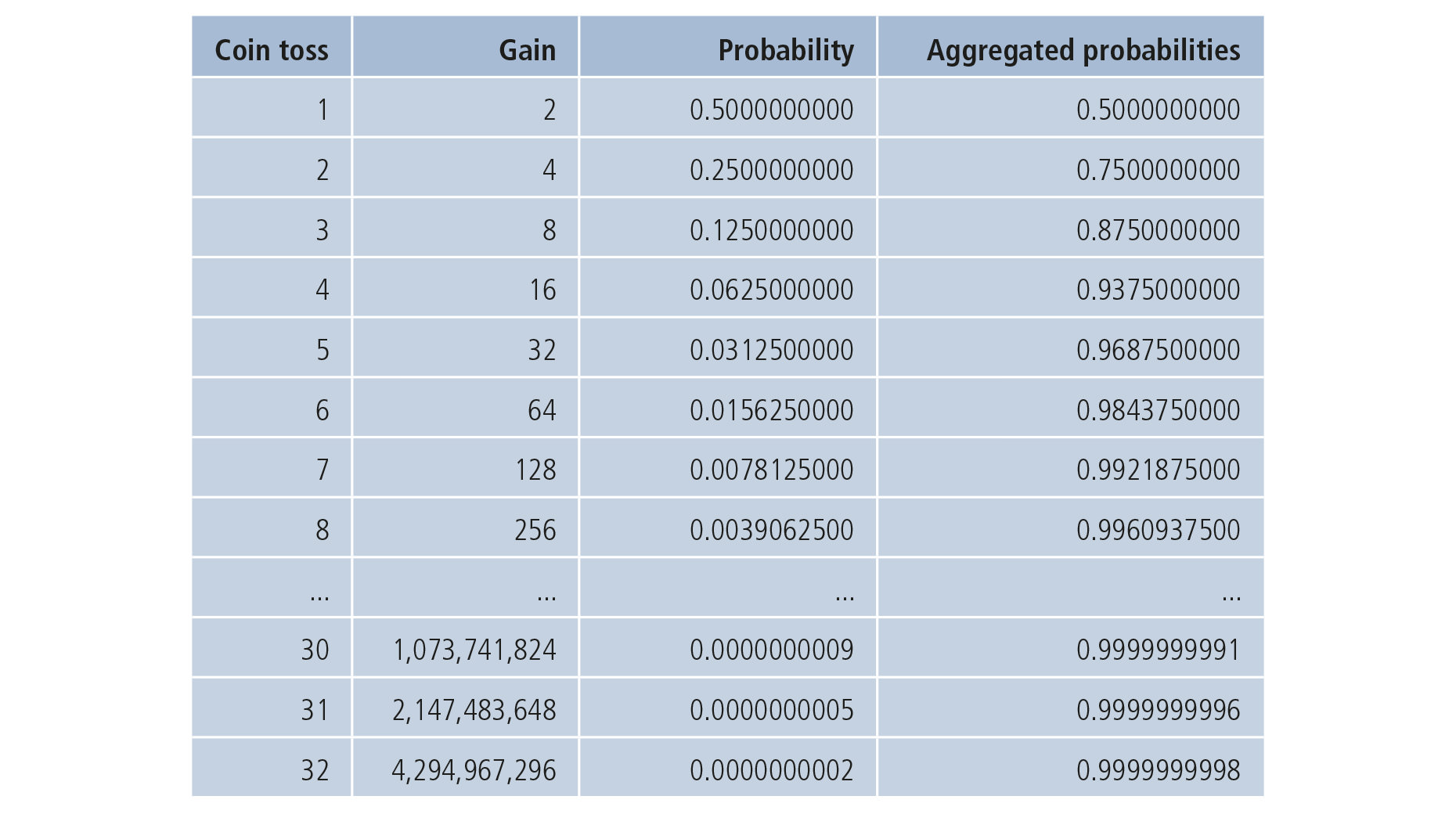
Figure 1 shows the gain achieved when tails appears for the first time after up to 32 tosses of the coin; the coin could be tossed this number of times in just a few minutes. The expected total payout for up to 32 coin tosses amounts to 32 = 25, as generally calculated above. We can see from the table, however, that the probability of actually achieving a gain equal to or greater than this value is fairly small – namely only 1 – 0.9375 = (½)4 = 0.0625 ≅ 6.25 per cent. As a general rule, the probability of achieving a gain of at least n = 2k is equal to (½)k-1, which means that it rapidly decreases towards zero as n increases. In other words, it is highly unlikely that players will achieve their expected gain (or more) in a St Petersburg lottery. Another way of putting it would be to say that the risk of not achieving their expected gain is very high.
In order to assess lottery competitions and investments, people have therefore devised methods which, instead of being based solely on the expected gain, also factor in risk measures or an assessment of individual utility for various levels of gains.
Mathematical and ‘real’ expected values
Events that are extremely unlikely would, in general, certainly not be ‘expected’. The term ‘expected value’, which has become widely used by scientists and academics to denote the probability-weighted mean, is therefore misleading – at least in the context of the lottery described above. Where did this term come from?
Events that are extremely unlikely would, in general, certainly not be ‘expected’
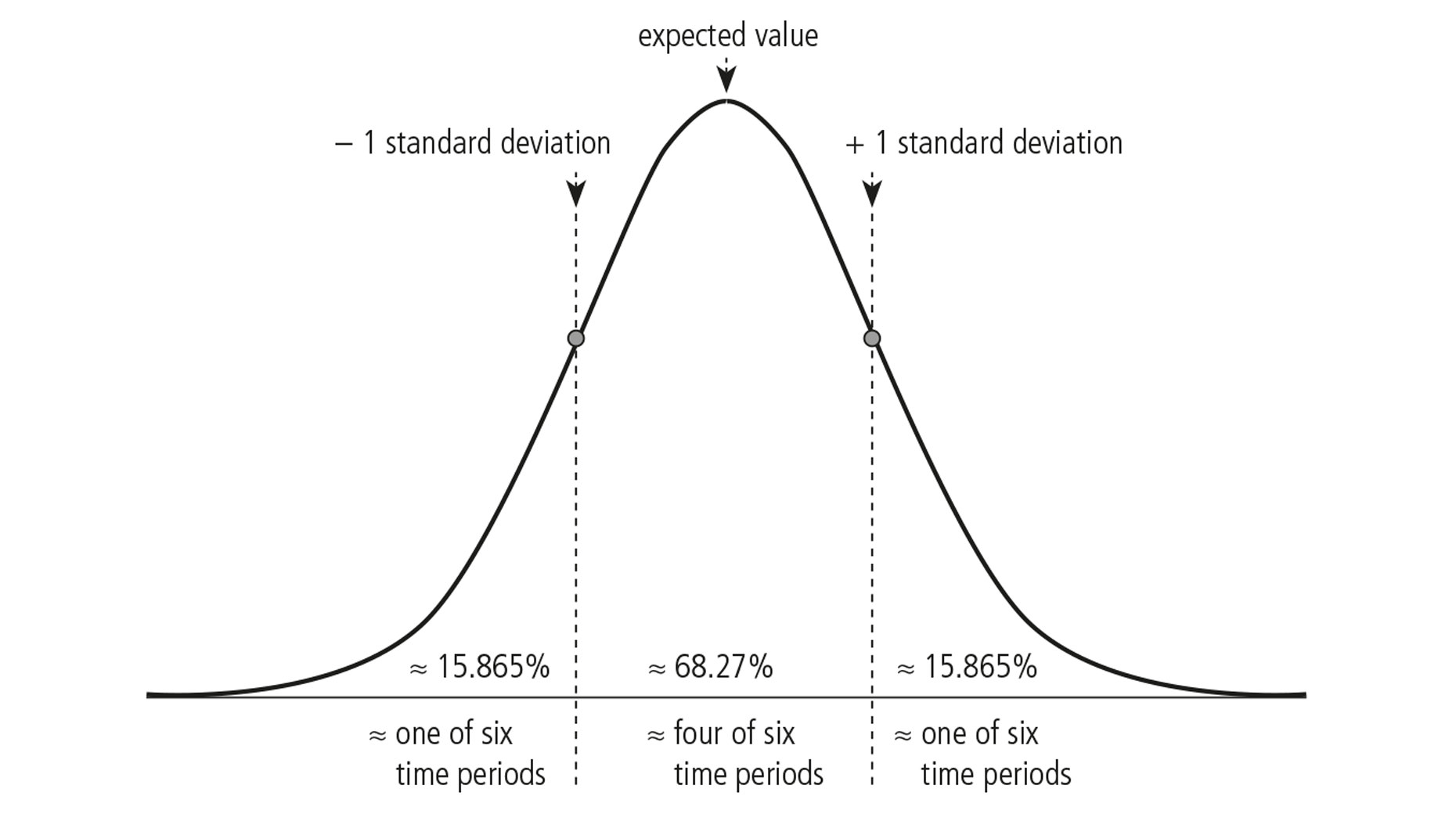
It is a well-established fact that normal distributions play an important role in random events. It can be mathematically demonstrated that normal distributions occur very frequently in the real world as at least approximate distribution models for random variables. However, this is usually the case – put simply – when numerous manifestations of these variables can be observed independently and almost simultaneously, as is often the case with the measurement results of physical experiments or with quantifiable characteristics such as the weight or height of individuals in a large population. In cases where there is a normal distribution, the expected value equals the maximum of the probability density function. The spread of the normal distribution is quantified by the so-called standard deviation. The probability mass, which lies within plus/minus one standard deviation of the expected value, amounts to approximately 68.27 per cent for any given normal distribution (see Figure 2).
In cases where there is a normal distribution or a similar distribution model, the mathematical expected value therefore behaves more or less as one would probably intuitively assume that such a number would do. However, the gain achieved in a St Petersburg lottery is anything but normally distributed.
Expected value of random returns
What can we say, then, about the probability distributions for random returns – such as those on equity portfolios? Can we not assume that they will exhibit something approaching a normal distribution? The answer is a resounding ‘no’ – at least if we are looking at the usual annualised rates of return (i.e. not at so-called continuously compounded returns). This is quite simply because – in theory, at least – infinitely large gains can be achieved (as in a St Petersburg lottery), whereas the downside loss is limited to 100 per cent, which would be the case if all the capital invested were wiped out.
Figure 3 shows a typical distribution of investment returns. In mathematical terms this is a shifted log-normal distribution. This type of distribution model occurs, for example, if the standard model of geometric Brownian motion is applied to share price performance. Other typical distribution models used for investment returns also behave – broadly speaking – in a similar way with respect to the parameters shown here (expected value, median, and maximum probability density).
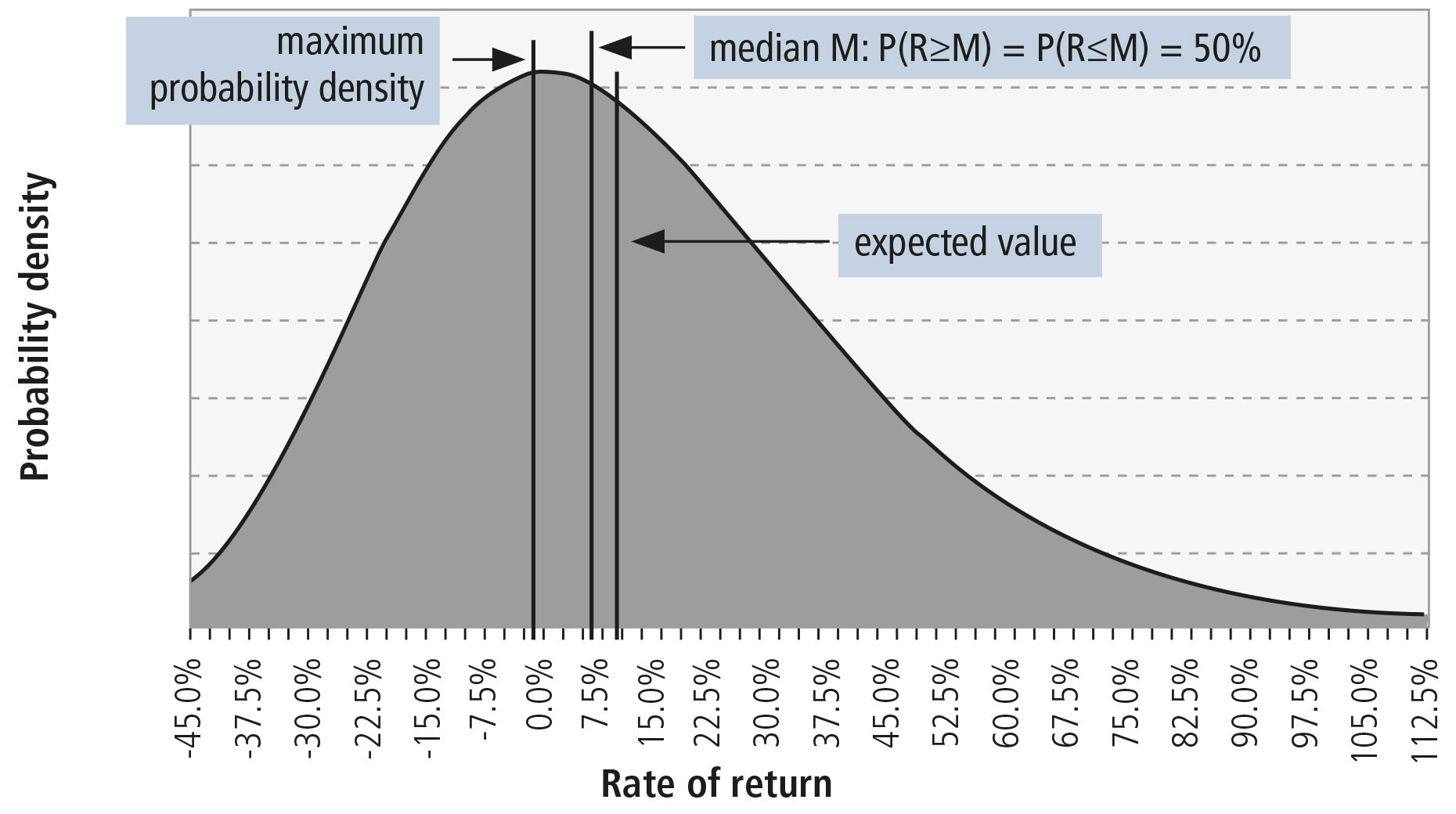
Unlike symmetrical normal distributions, such distributions are skewed to the right; this means that the expected value lies to the right of the median. The median of a probability distribution is defined as the value above which 50 per cent of the probability mass lies and below which 50 per cent of this mass lies.
The expected value says very little about the ‘probable rates of return’
This means, in statistical terms, that the expected value is actually achieved in fewer than 50 per cent of all investment years. The maximum density, whose surrounding area one would probably intuitively assume – based on the chart – to be the ‘expected return’ field, actually lies to the left of the median in the area of even lower returns. The greater the variance of values overall – in other words, to put it simply, the greater the investment risk – the greater the differences between the aforementioned values.
The high expected return arises only because the calculation of the mean includes ‘improbably high’ positive returns of well over 100 per cent, for example, whereas negative returns are limited to 100 per cent. Although – as far as random returns on investments are concerned – achieving at least the expected return is typically nowhere near as unlikely as in a St Petersburg lottery, those looking to assess their risks accurately should be aware that the expected value says very little about the rates of return that ‘can probably be achieved’.
About the author
After completing her PhD in mathematics and then carrying out post-doctoral research, Claudia Cottin, born 1958, worked for several years in the insurance industry, where she qualified as an actuary by passing the German Actuarial Association (DAV) exams. She is currently professor of financial and actuarial mathematics at Bielefeld University of Applied Sciences and is a regular visiting professor at City University of Hong Kong. Among her many publications she has co-authored a textbook on risk analysis (Risikoanalyse), which is published by Springer-Verlag.